
Post 5 (Image Classification with Tensorflow)
Let’s use Tensorflow to teach a machine learning algorithm to distinguish between pictures of dogs and pictures of cats!
Here is the post’s general layout:
- Before Start
- A. First Model
- B. Model with Data Augmentation
- C. Data Preprocessing
- D. Transfer Learning
- Score on Test Data
Before Start
Let’s first import all the packages we need!
import os
import tensorflow as tf
from tensorflow.keras import utils, datasets, layers
import matplotlib.pyplot as plt
import numpy as np
Next, copy and paste the following code to access the data provided by Tensorflow team.
# location of data
_URL = 'https://storage.googleapis.com/mledu-datasets/cats_and_dogs_filtered.zip'

# download the data and extract it
path_to_zip = utils.get_file('cats_and_dogs.zip', origin=_URL, extract=True)

# construct paths
PATH = os.path.join(os.path.dirname(path_to_zip), 'cats_and_dogs_filtered')

train_dir = os.path.join(PATH, 'train')
validation_dir = os.path.join(PATH, 'validation')

# parameters for datasets
BATCH_SIZE = 32
IMG_SIZE = (160, 160)

# construct train and validation datasets
train_dataset = utils.image_dataset_from_directory(train_dir,
                                                   shuffle=True,
                                                   batch_size=BATCH_SIZE,
                                                   image_size=IMG_SIZE)

validation_dataset = utils.image_dataset_from_directory(validation_dir,
                                                        shuffle=True,
                                                        batch_size=BATCH_SIZE,
                                                        image_size=IMG_SIZE)

# construct the test dataset by taking every 5th observation out of the validation dataset
val_batches = tf.data.experimental.cardinality(validation_dataset)
test_dataset = validation_dataset.take(val_batches // 5)
validation_dataset = validation_dataset.skip(val_batches // 5)
Now we have created our Tensorflow datasets for training, validation, and testing.
It is called “datasets” because we will be conducting machine learning in batches, so that we wouldn’t overload our memory. Parameter BATCH_SIZE provides the size of each batch. Here we have 32 images in each batch.
Then we used image_dataset_from_directory() to create these datasets, and separated them into train_dataset and validation_dataset.
Next, let’s copy and paste the following code to use “AUTOTUNE” to prefetch our datasets. The purpose of this step is to improve the reading time.
AUTOTUNE = tf.data.AUTOTUNE

train_dataset = train_dataset.prefetch(buffer_size=AUTOTUNE)
validation_dataset = validation_dataset.prefetch(buffer_size=AUTOTUNE)
test_dataset = test_dataset.prefetch(buffer_size=AUTOTUNE)
Examine the Datasets
Working with Tensorflow Datasets
To get one “batch” from the datasets, we can use the take() function. For example, train_dataset.take(1) will retrieve one batch (32 images with labels) from the training data.
Let’s explore the dataset a little! To do this, let’s create some visualization of the pictures in one dataset.
# create plot
plt.figure(figsize=(10, 10))
# take one batch from the datasets
dataset = train_dataset.take(1)

def plot_images(dataset):
  # let's create 2 rows of pictures,
  # with 3 pictures from each label
  for images, labels in dataset:
    # first row
    for i in range(3):
      # take random index until find a cat
      pic = np.random.randint(32)
      ax = plt.subplot(2, 3, i + 1)
      while(labels[pic]!=0):
        pic = np.random.randint(32)
      # plot the cat
      plt.imshow(images[pic].numpy().astype("uint8"))
      plt.title("cats")
      plt.axis("off")

    #second row
    for i in range(3,6):
       # take random index until find a dog
      pic = np.random.randint(32)
      ax = plt.subplot(2, 3, i + 1)
      while(labels[pic]!=1):
        pic = np.random.randint(32)
      # plot the dog
      plt.imshow(images[pic].numpy().astype("uint8"))
      plt.title("dogs")
      plt.axis("off")

plot_images(dataset)
output:
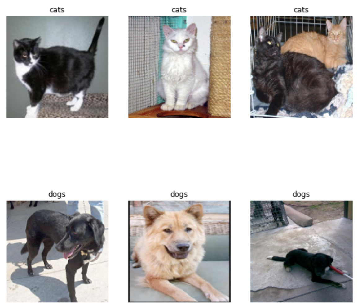
From our two-row visualization, we can see what kind of images are included in the datasets.
Check Label Frequencies
Copy and paste the following code to create an iterator called labels:
labels_iterator= train_dataset.unbatch().map(lambda image, label: label).as_numpy_iterator()
Let’s compute each label’s frequency:
# variables to store the count
dog_count = 0
cat_count = 0

# increment the count variable as we iterate
for label in labels_iterator:
  if (label==0):
    cat_count +=1
  else:
    dog_count +=1

print(dog_count, cat_count)
output:
1000 1000
The baseline machine learning model is the model that always guesses the most frequent label. Since each label is equally frequent, our baseline should be 50%.
Thus, the baseline should be 50% accurate in our model.
Let’s treat this as a benchmark for evaluating the performence of our models!
A. First Model
We’ll be using the following functions to help us build our first model!
We will be building a Convoluted Neural Network (CNN) model, which is an artificial neural network (ANN) with multiple layers between the input and output layers.
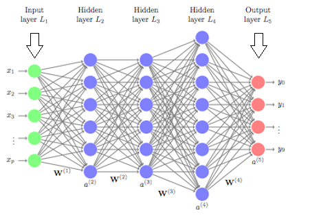
In Machine Learning classification problem, we learn parameters to generalize the features of each class. In Deep Neural Network (DNN), each layer composes of the features that we learned, and we do this multiple times to derive information.
CNN is a special type of DNN. It is great for image classification, as it learns patterns in images that are ‘shift-invariant’. In addition, it not only recognizes patterns from images, but also abstracts such patterns (ex. learns the edges, color then larger shapes in the next layer, etc).
CNN is usually composed of two types of layers: convolution layer and pooling layer.
tf.keras.models.Sequential() is an API that allows you to construct a model by simply passing a list of layers. We can use it as follows: model = tf.keras.models.Sequential([ # layer 1, # layer 2 … # layer N ])
tf.keras.layers.Conv2D: this layer creates the convolution layer for CNN. It takes parameters such as number of filters, kernel size, activation method, etc. It learns filters from the data, and each filter is supposed to capture a particular pattern everywhere in the image.
tf.keras.layers.MaxPooling2D: this layer creates the pooling layer for CNN. It takes parameters such as the size of each pooling layer. It is used to reduce the size of the previous layer’s output by either keeping the most dominant cell value in each patch (called ‘max-pool’) or averaging every patch into a single scalar (called ‘avg-pool’).
tf.keras.layers.Dropout: this layer can help us reduce overfitting by using regularizer to ignore some units! We can simply use it by passing a rate parameter, thus it randomly sets input units to 0 with the rate we passed in at each step during training time.
tf.keras.layers.Flatten: this layer simply flattens the input, because for our classification, we want a array of values to make prediction for each data point.
tf.keras.layers.Dense: we use this layer to sum up of the parameters we have so far. When it is supplied with the “softmax” function, we’re transforming the parameters into a set of probability of each class for a single data point. For example, if we have tf.keras.layers.Dense(2, activation=’sigmoid’), we will have 2 probabilities for each data point, say [0.4, 0.6]: then the probability that the data point is labeled 0 is 0.4, and the probability for labeled 1 is 0.6.
We use the loss function to calculate the loss of information at each step, and the optimization algorithm to minimize the loss, such that our algorithm can learn to classify correctly. Thus, before we run the model, we need to specify the loss function and the optimization algorithm. We do so by compiling the model with the compile() function.
We can also see how many parameters are being learned at each layer using the summary() function.
Now we have learned all the tools we can use to construct a CNN model. Let’s build one!
model1 = tf.keras.models.Sequential([
    # first Conv.+ReLu with Max-Pool
    layers.Conv2D(16, 3, activation='relu', input_shape=(160, 160, 3)),
    layers.MaxPooling2D(2),

    # second Conv.+ReLu with regularizer and Max-Pool
    layers.Conv2D(32, 3, activation='relu'),
    layers.Dropout(0.3),
    layers.MaxPooling2D(2),

    # change the shape of parameters
    layers.Flatten(),
    # densen parameters
    layers.Dense(64, activation='relu'),
    # get probabilities
    layers.Dense(2, activation='sigmoid')
])

model1.compile(optimizer='adam',
              loss='sparse_categorical_crossentropy',
              metrics=['accuracy'])

model1.summary()
output:
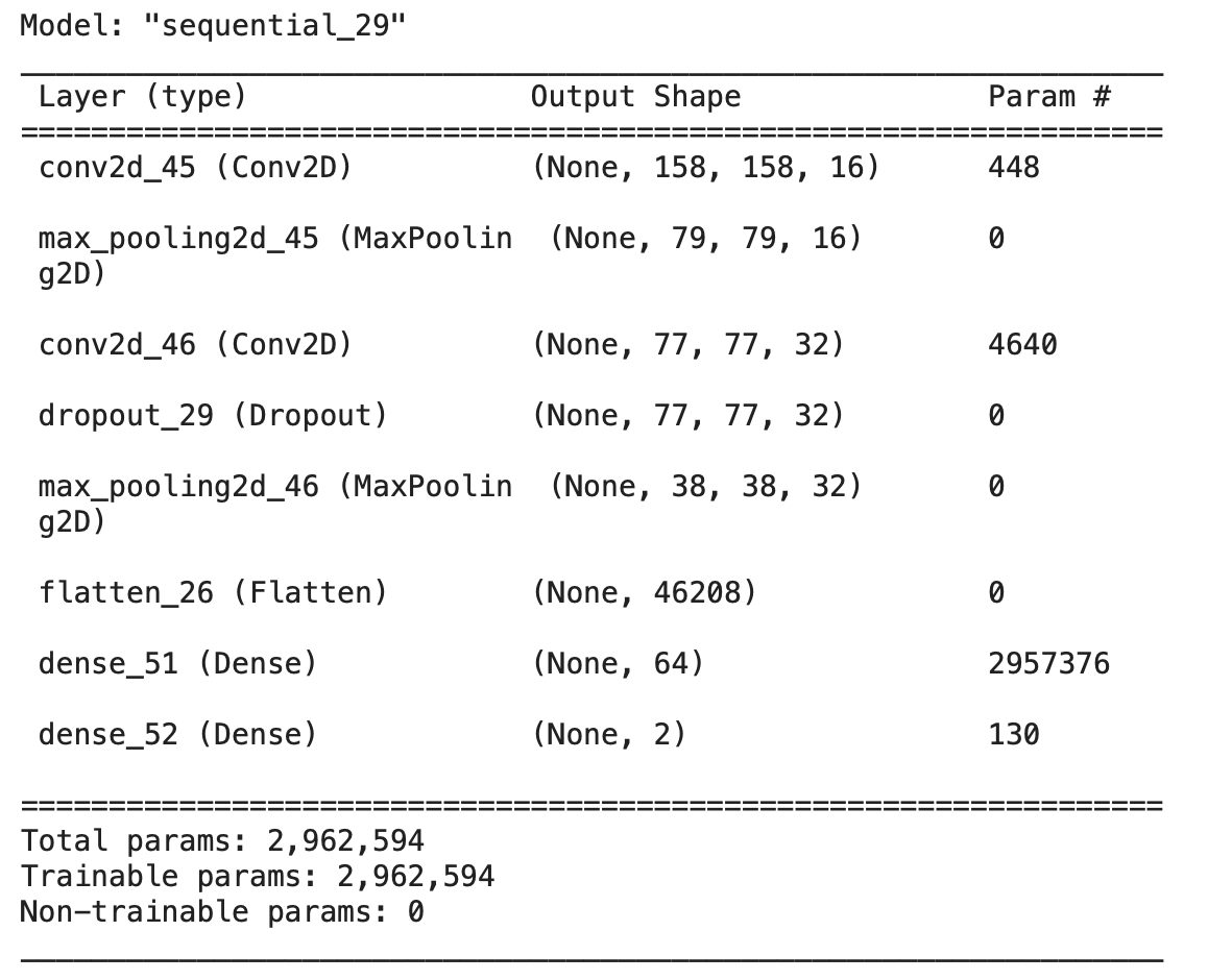
We can try a few different parameters/layers to get better accuracy. For example, I tried 2 Conv2D(32, 9) and 2 MaxPooling2D(4); 2 Conv2D(32, 6) and 2 MaxPooling2D(2); etc. After a few trials, I found out that Conv2D(16, 3), Conv2D(32, 3) and and 2 MaxPooling2D(2) works fine for this model.
Next, let’s train the model on the datasets!
Model Training: we will be passing in 3 parameters:
-
training_data;
-
epoch: this is the number of rounds through the data that the model is going to do;
-
validation_data;
Our code looks like this:
history = model1.fit(train_dataset,
# run the model 20 times
epochs=20,
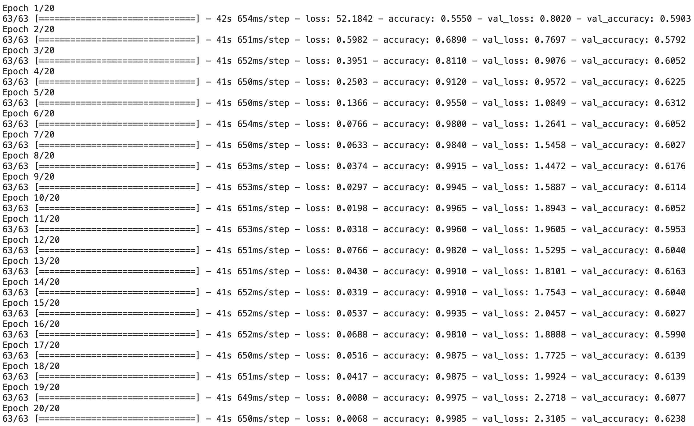
validation_data=validation_dataset)
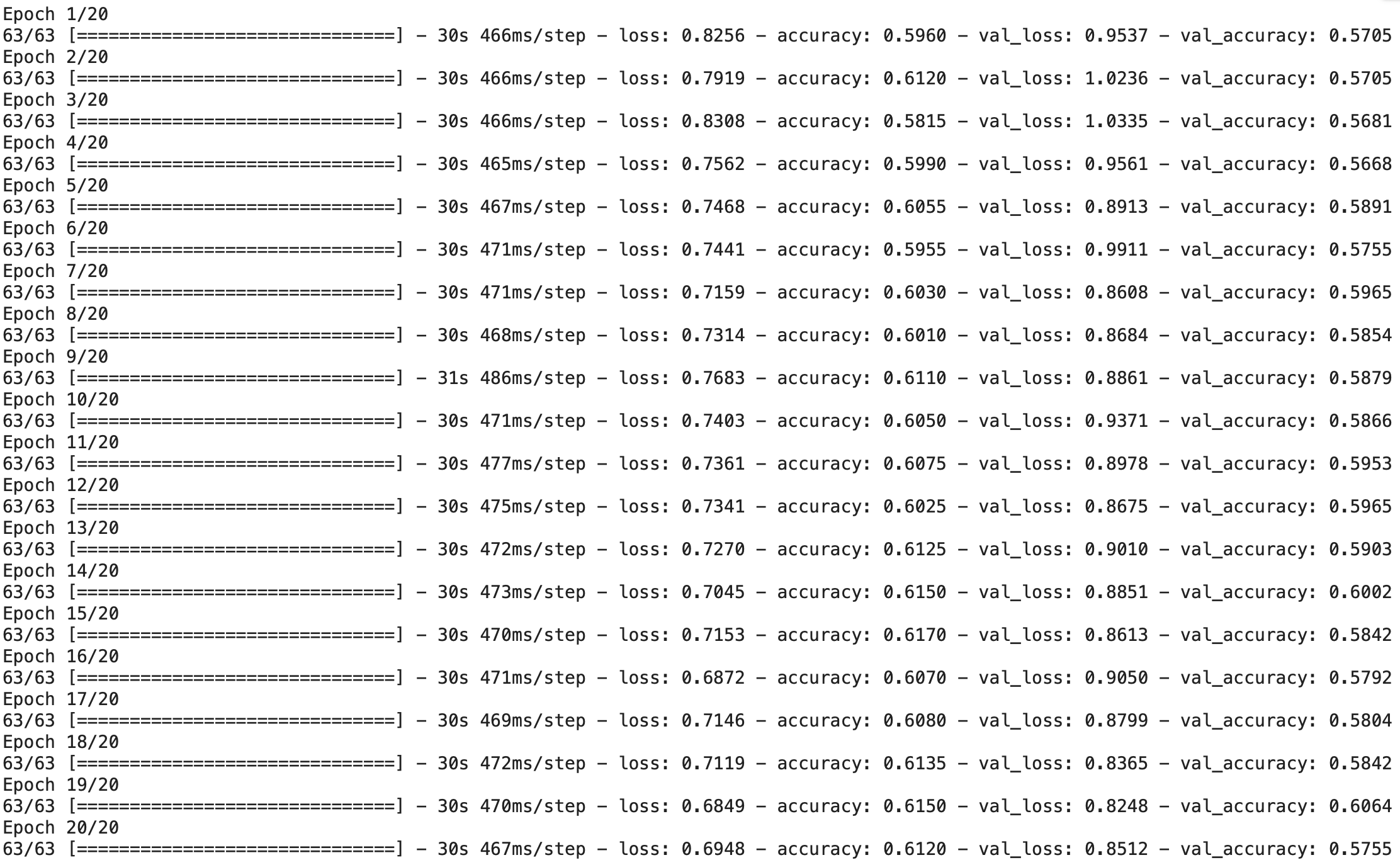
output:
Let’s plot the model accuracy for training data and validation data:
plt.plot(history.history['accuracy'], label="training")
plt.plot(history.history['val_accuracy'], label="validation")
plt.gca().set(xlabel="epoch", ylabel="accuracy", title="accuracy comparison")
plt.legend()
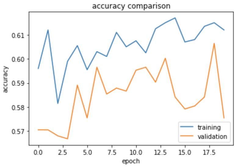
output:
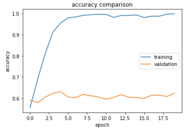
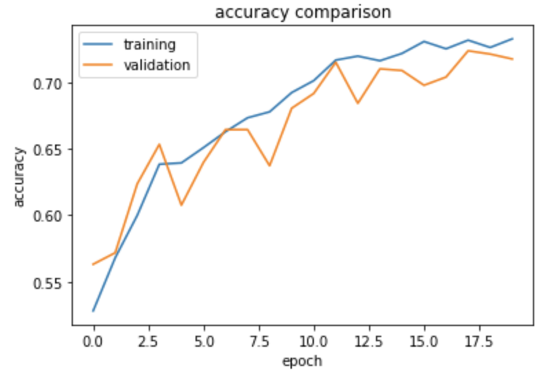
The accuracy of this model stabilized between 60% and 63% during training. This is around 10% higher than the baseline.
From the graph above, we can tell that the training accuracy is much higher than the validation accuracy. There is probably some overfitting!
B. Model with Data Augmentation
In this section, we will be using two new types of layers:
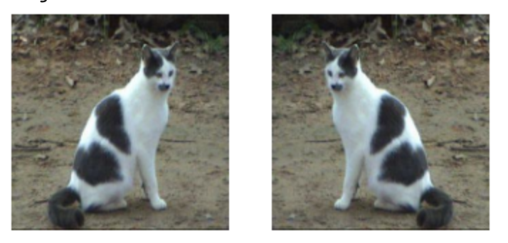
tf.keras.layers.RandomFlip(): this layer randomly flips images (horizontally or vertically). Let’s examine this layer with the following code:
random_flip = layers.experimental.preprocessing.RandomFlip()
# create plot
plt.figure(figsize=(10, 10))
for images, labels in train_dataset.take(1):
      # take a random picture
      pic = np.random.randint(32)
      # create 2 pictures one 1 row
      fig, ax = plt.subplots(1, 2)
      # the original image
      ax[0].imshow(images[pic].numpy().astype("uint8"))
      ax[0].axis("off")
      # the fandomly flipped image
      ax[1].imshow(random_flip(images[pic]).numpy().astype("uint8"))
      ax[1].axis("off")
tf.keras.layers.RandomRotation(): this layer randomly rotate images, and we can pass in a float to represent a fraction of 2 Pi (i.e. degree of rotation). Let’s examine this layer with the following code:
random_rotate = layers.RandomRotation(0.2)
# create plot
plt.figure(figsize=(10, 10))
for images, labels in train_dataset.take(1):
      # take a random picture
      pic = np.random.randint(32)
      # create 2 pictures one 1 row
      fig, ax = plt.subplots(1, 2)
      # the original image
      ax[0].imshow(images[pic].numpy().astype("uint8"))
      ax[0].axis("off")
      # the fandomly rotated image
      ax[1].imshow(random_rotate(images[pic]).numpy().astype("uint8"))
      ax[1].axis("off")
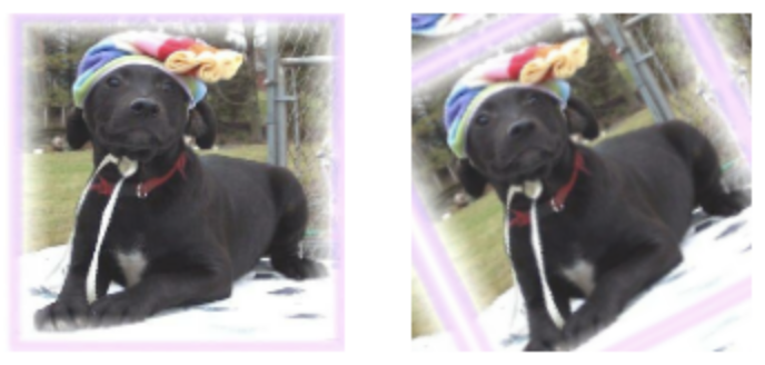
These are 2 types of data augmentation layers. Data Augmentation means to do some changes to our data, such as the flipping and rotating above, so that we can have greater diversity in our dataset.
In this model, we wish to add these 2 data augmentation layers, so that our algorithm can be learning actural features:
model2 = tf.keras.Sequential([
# augmentation layers
layers.experimental.preprocessing.RandomFlip(),
layers.experimental.preprocessing.RandomRotation(0.2),
# Conv.+ReLu with Max-Pool
layers.Conv2D(16, 3, activation='relu', input_shape=(160, 160, 3)),
layers.MaxPooling2D(2),
# change the shape of parameters
layers.Flatten(),
# densen parameters
layers.Dense(64, activation='relu'),
# get probabilities
layers.Dense(2, activation='sigmoid')
])
model2.compile(optimizer='adam',
loss='sparse_categorical_crossentropy',
metrics=['accuracy'])
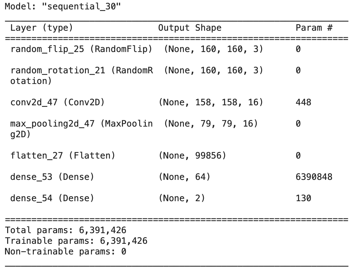
model2.summary()
output:
Train the algorithm as in section A:
history = model2.fit(train_dataset,
                    # run the model 20 times
                     epochs=20,
                     validation_data=validation_dataset)
Let’s plot the model accuracy for training data and validation data:
plt.plot(history.history['accuracy'], label="training")
plt.plot(history.history['val_accuracy'], label="validation")
plt.gca().set(xlabel="epoch", ylabel="accuracy", title="accuracy comparison")
plt.legend()
output:
The accuracy of this model stabilized between 57% and 60% during training. Our accuracy actually decreased by 3% compared to Model1!
However, the gap between the training accuracy and the validation accuracy is a lot smaller than in model 1. There is probably still some overfitting, but a lot better than in model 1!
C. Data Preprocessing
Let’s keep improving our model! In this step, we’re going to simply transform the input data. For example, we can normalize the RGB value 0→225 to 0→1 or -1→1. By doing so, we can focus on handling the actual signal of the input data!
Let’s create a preprocessor with the following code:
i = tf.keras.Input(shape=(160, 160, 3))
x = tf.keras.applications.mobilenet_v2.preprocess_input(i)
preprocessor = tf.keras.Model(inputs = [i], outputs = [x])
With this layer, our input data can be modified. We can use this as the first layer of our new model:
model3 = tf.keras.Sequential([
    # the preprocessing layer implemented above
    preprocessor,

    # augmentation layers
    layers.experimental.preprocessing.RandomFlip(),
    layers.experimental.preprocessing.RandomRotation(0.2),

    # Conv.+ReLu with Max-Pool
    layers.Conv2D(16, 3, activation='relu', input_shape=(160, 160, 3)),
    layers.MaxPooling2D(2),
    layers.Conv2D(32, 3, activation='relu'),
    layers.MaxPooling2D(2),

    # change the shape of parameters
    layers.Flatten(),
    # densen parameters
    layers.Dense(64, activation='relu'),
    # get probabilities
    layers.Dense(2, activation='sigmoid')
  ])

model3.compile(optimizer='adam',
              loss='sparse_categorical_crossentropy',
              metrics=['accuracy'])
model3.summary()
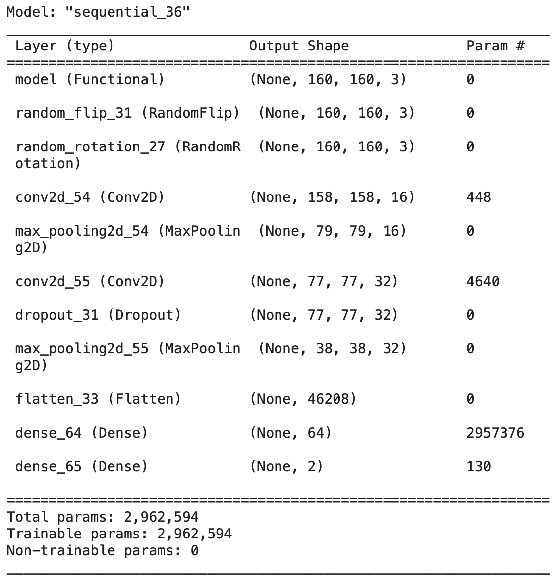
output:
Train the algorithm as in section A:
history = model3.fit(train_dataset,
                    # run the model 20 times
                     epochs=20,
                     validation_data=validation_dataset)
Let’s plot the model accuracy for training data and validation data:
plt.plot(history.history['accuracy'], label="training")
plt.plot(history.history['val_accuracy'], label="validation")
plt.gca().set(xlabel="epoch", ylabel="accuracy", title="accuracy comparison")
plt.legend()
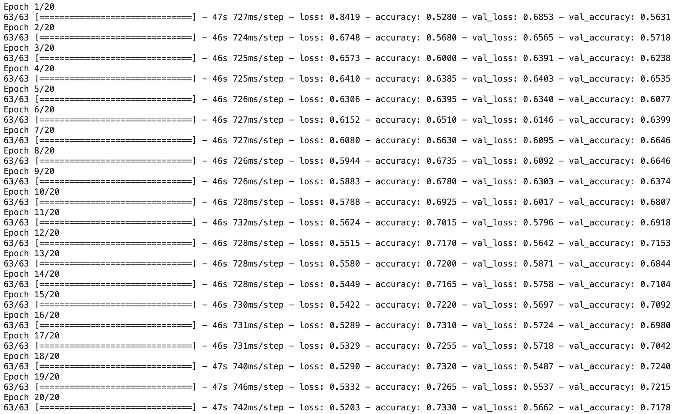
output:
The accuracy of this model stabilized between 70% and 72% during training. Our accuracy has improved significantly from model1!
There is now no apparent gap between the training accuracy and the validation accuracy. We can say that there is probably little or no overfitting!
D. Transfer Learning
While we’re doing image classification, someone else might be doing it too! People might have learned some patterns from their training, and we can actually use that for our model!
Copy and paste the following code to download MobileNetV2 and use it as a base model layer in our model:
IMG_SHAPE = IMG_SIZE + (3,)
base_model = tf.keras.applications.MobileNetV2(input_shape=IMG_SHAPE,
                                               include_top=False,
                                               weights='imagenet')
base_model.trainable = False

i = tf.keras.Input(shape=IMG_SHAPE)
x = base_model(i, training = False)
base_model_layer = tf.keras.Model(inputs = [i], outputs = [x])
Now let’s create our final model with the base model layer created above!
model4 = tf.keras.Sequential([
# the preprocessing layer implemented above
preprocessor,
# augmentation layers
layers.experimental.preprocessing.RandomFlip(),
layers.experimental.preprocessing.RandomRotation(0.2),
# got this from MobileNetV2
base_model_layer,
# some pooling and dropouts
layers.GlobalMaxPooling2D(),
layers.Dropout(0.3),
# change the shape of parameters
layers.Flatten(),
# densen parameters
layers.Dense(64, activation='relu'),
# get probabilities
layers.Dense(2, activation='sigmoid')
])
model4.compile(optimizer='adam',
loss='sparse_categorical_crossentropy',
metrics=['accuracy'])
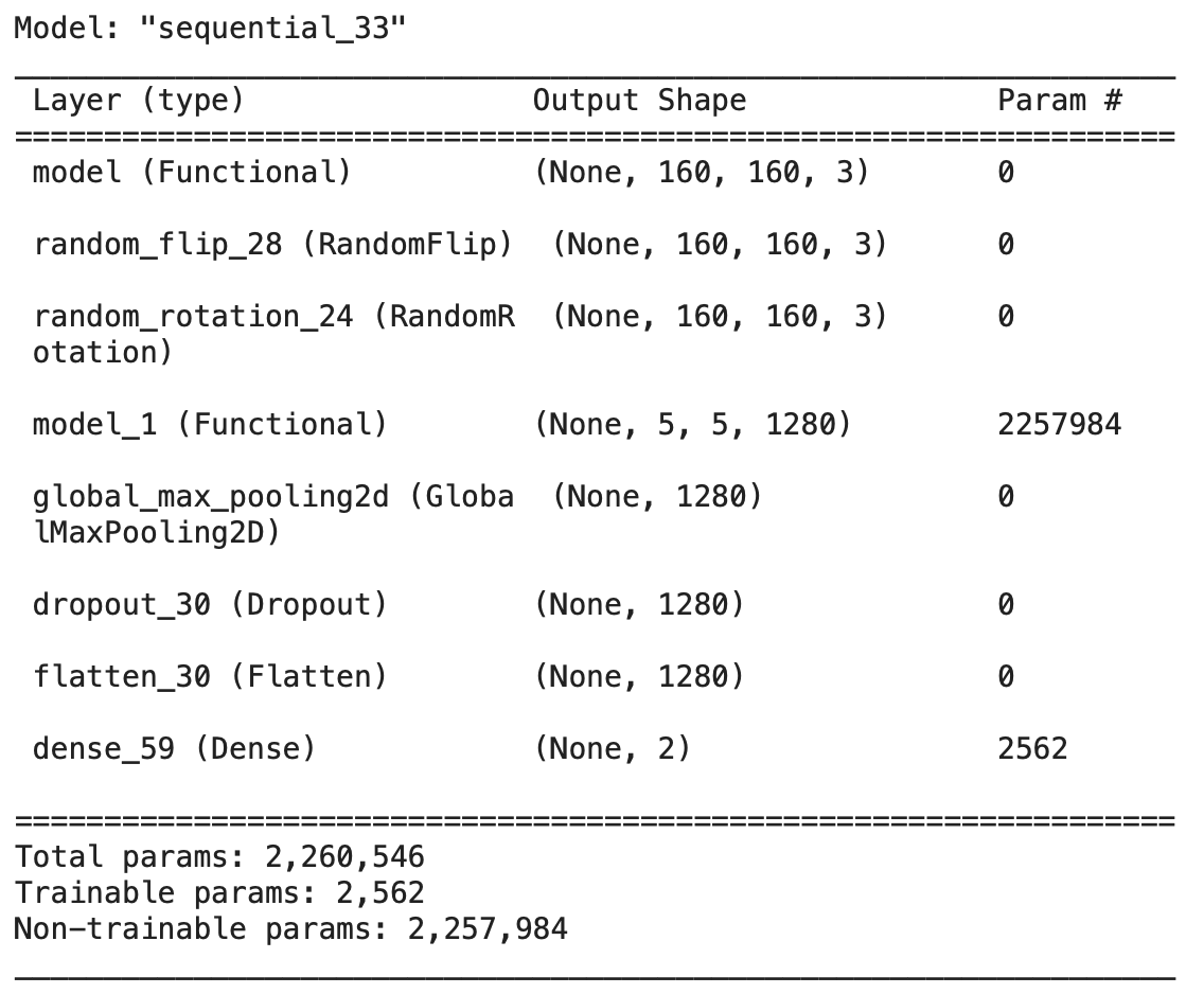
model4.summary()
output:
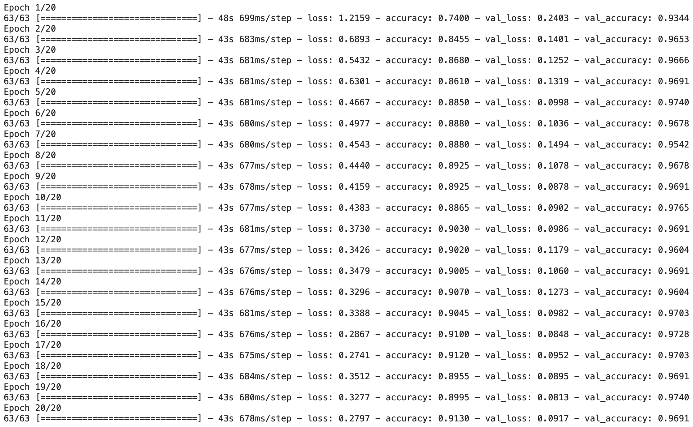
Train the algorithm as in section A:
history = model4.fit(train_dataset,
                    # run the model 20 times
                     epochs=20,
                     validation_data=validation_dataset)
Let’s plot the model accuracy for training data and validation data:
plt.plot(history.history['accuracy'], label="training")
plt.plot(history.history['val_accuracy'], label="validation")
plt.gca().set(xlabel="epoch", ylabel="accuracy", title="accuracy comparison")
plt.legend()
output:
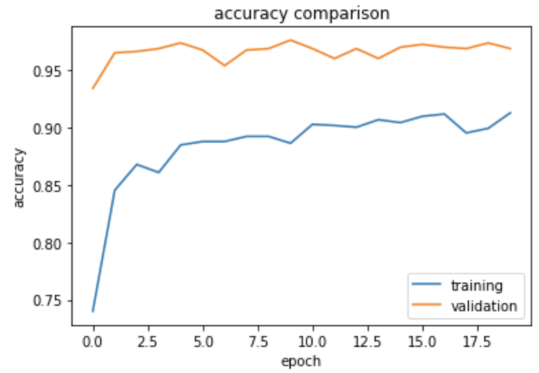
The accuracy of this model stabilized between 96% and 97% during training. Our accuracy is a lot better than any models we created before!
There is also no apparent overfitting pattern now: as training accuracy improves, the validation accuracy slowly improves too; validation accuracy actually gets higher than the training accuracy, and the gap between the accuracies are small.
Score on Test Data
Finally, let’s evaluate the accuracy of Model 4 on the testing dataset!
model4.evaluate(test_dataset)
output:

We have a 95% accuracy on classifying the dataset!