We usually use the sklearn.cluster.KMeans function to identify clusterings in a dataset.
However, when your clusters aren’t blobs (for example, moons or rings), this function can hardly identify your clusters.
Thus, let’s implement an algorithm to identify difficult clusters!

Here is the post’s general layout:

• Before Start
• A. Construct a Similarity Matrix
• B. Calculate Norm Cut
• C. Another Way to Approach Norm Cut
• D. Optimization Based On Part C
• E. Check the Partition From Part D
• F. Optimize with Eigenvalues and Eigenvectors
• G. Synthesize Everything
• H. Testing
• I. Challange!

Before Start

Before we start implementing the algorithm, let’s check the format of our data:

# import packages
import numpy as np
from sklearn import datasets

# create dataset
n = 200
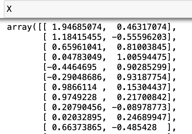
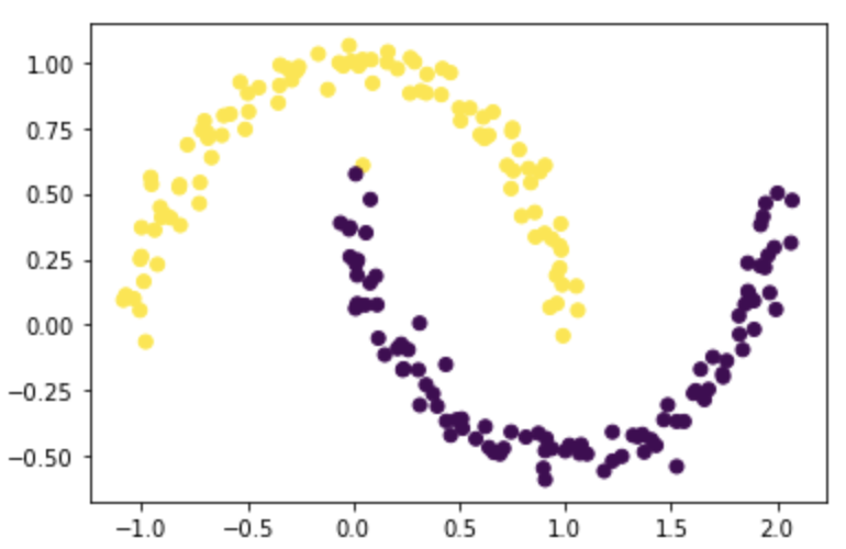
X, y = datasets.make_moons(n_samples=n, shuffle=True, noise=0.05, random_state=None)

\(X\) is a nx2 numpy array; each row represents a data point, and the two values in each row represents the position (x,y) of the data point on the 2D plane

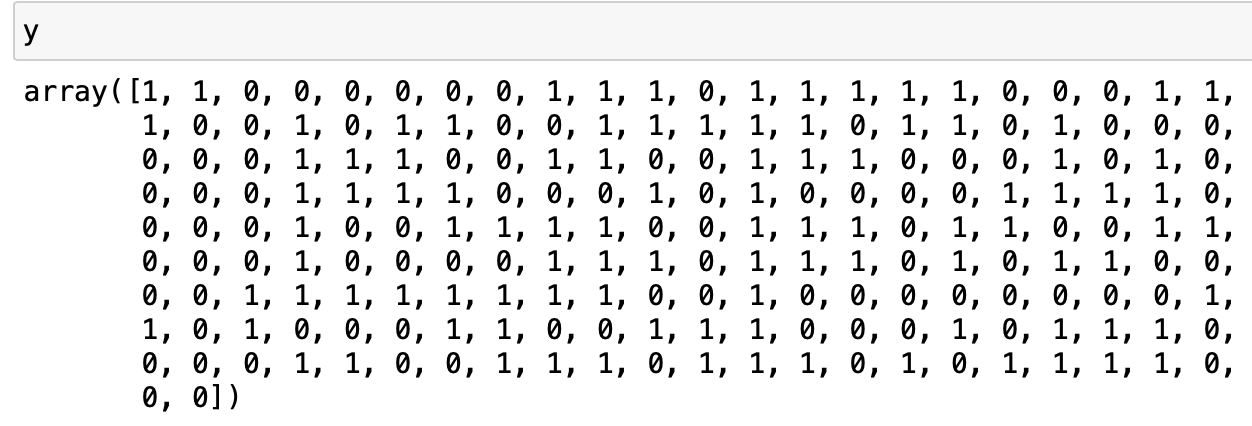
\(y\) is a length n numpy array; it is composed of 0 and 1, representing the two groups each data point belongs to

A. Construct a Similarity Matrix

In math, two points are considered close to each other if the distance between them is smaller than some epsilon \(\epsilon > 0\).
We wish to construct a distance matrix A with shape nxn, such that A[i,j] represents the distance d[i,j] between point X[i] and X[j].
We can achieve this by the function pairwise_distances from sklearn.metrics:

# import package
from sklearn.metrics import pairwise_distances

# create a distance matrix with sklearn function
A = pairwise_distances(X)

Next, let’s change this distance matrix into a similarity matrix:

1. if d[i,j] is less than our chosen epsilon, then A[i,j] is 1 (meaning these two points are close to each other)
2. else, A[i,j] is 0 (meaning these two points are not close)
3. we also want all diagonal entries of A to be 0.

# choosing epsilon
epsilon = 0.4

# change entry values according to the rules
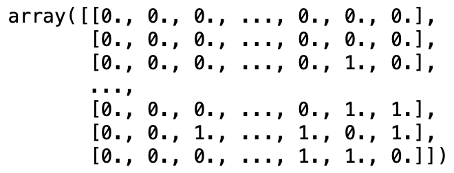
A = 1*(A < epsilon)
np.fill_diagonal(A, 0)

A

output:

B. Calculate Norm Cut

Now we can separate the data points in B by partitioning the rows and columns of A!

Say that there are 2 clusters, call them \(C_0\) and \(C_1\). Then each point in X is either in \(C_0\) or \(C_1\). The cluster “membership” corresponds to the y labeling we mentioned earlier.

Where
\(cut_{C_0, C_1} = \sum_{i \in C_0, j \in C_1} A_{ij}\)
\(vol_{C_0} = \sum_{i \in C_0}d_i = \sum_{i \in C_0}\sum_j A_{ij}\)
\(vol_{C_1} = \sum_{i \in C_1}d_i = \sum_{i \in C_1}\sum_j A_{ij}\)

Note 1: cut is the sum of all entries (also the non-zero entries) that relates points in different clusters.
Note 2: vol is the sum of degrees of all points in one cluster.

1. The Cut Term

Let’s first write a function to calculate the cut between two clusters.

def cut(A,y):
  # initialize the cut value
  cut = 0

  # iterate through all pairs of [i,j]
  for i in range(n):
    for j in range(i,n):
      # add value A[i,j] to the cut if 
      # the two points belong to different clusters
      if y[i]!=y[j]:
        cut += A[i,j]
  return cut

Let’s try it on our true labels:

cut(A,y)

output: 13.0

Let’s also try it on some fake labels:

# create fake labels
fake_label = np.random.randint(2, size=n)
cut(A,fake_label)

output: 1094.0

By definition of cut, the more correct your labeling is, the more distance between the points from each cluster, thus the smaller cut should be.
From the example above, we can see that cut does favor the true labels over the fake ones.

2. The Volume Term

Let’s now write a function to calculate the vol of each cluster.

def vols(A,y):
  # boolean arrays for each cluster
  C0 = (y==0)
  C1 = (y!=0)
  # A[C0] and A[C1] select points from each cluster,
  # and sum() sums up the degree of each point,
  # and then sums up all degrees
  return A[C0].sum(), A[C1].sum()

Note: degree determines whether a point is close to all other points.
The greater the degree, the more points it is close to.
Since it only sums up the degree of points in one cluster, it calculates the “size” of a cluster.

3. Calculate Norm Cut

We can now calculate the norm cut based on the functions in 1 and 2!

def normcut(A,y):
  # calculate cut, vol(c0), vol(c1)
  cut_ = cut(A,y)
  v0, v1 = vols(A,y)

  # calculate norm cut based on the equation
  return cut_ * (1/v0 + 1/v1)

The smaller the norm cut, the better our partition is.

Note: by definition of norm cut, to have a good partition, we want a small cut and big vols.
This makes sense, as discussed in part 1: the smaller the cut, the better the partition.
Also in part 2: the bigger the vol, the bigger the cluster. This ensures that we don’t have clusters that are too small.

Let’s try it on our true labels:

normcut(A, y)

output: 0.011518412331615225

Let’s also try it on some fake labels:

# create fake labels
fake_label = np.random.randint(2, size=n)
cut(A,fake_label)

output: 0.9843523861136791

The norm cut for fake labels is greatly larger than the norm cut for true labels. This matches our expectation!

C. Another Way to Approach Norm Cut

Now we have a measure for how good our partition is! We can try to find a y such that normcut(A, y) is small, then this y will be a good labeling of our clusters!

However, this is a hard optimization problem to solve. Thus, we can do some linear algebra to transform the formula ① \(cut_{C_0, C_1}(\frac{1}{vol_{C_0}} + \frac{1}{vol_{C_1}})\) into formula ② \(\frac{z^T (D - A)z} {z^T D z}\),
where D is the diagnonal matrix with diagonal entries \(d_{ii} = \sum_{j = 1}^n a_i\),
\(z_i = \frac{1}{vol_{C_0}}\) if \(y_i = 0\); \(z_i = -\frac{1}{vol_{C_1}}\) otherwise.
Since z contains all information from y, we can now try to find a z such that the value of formula ② is small. This is a much better optimization problem to solve!
Let’s try to implement this, and see whether these two formulas are equivalent!

1. Compute z

Let’s write a transform function to compute z:

def transform(A,y):
  # initialize z and volumes
  z = np.zeros(n)
  v0, v1 = vols(A,y)

  # calculate z based on the formula
    for i in range(n):
        if y[i]==0:
            z[i] = 1/v0
        else:
            z[i] = -1/v1
    return z
z = transform(A,y)

2. Compute D

Let’s compute D according to the formula above:

# initialize D
D = np.zeros((n,n))
# fill the diagonals with sum of each row in A (degree)
np.fill_diagonal(D, sum(A[:,]))

3. Check Calculation

Let’s first check whether we implemented the functions right.
It we did it correctly, we should have \(\mathbf{z}^T\mathbf{D}\mathbb{1} = 0\)

# check whether z and D are implemented correctly
z @ D @ np.ones(n)

output: 0.0

Next, let’s check whether formula ① and ② are equivalent on our current A and y:

np.isclose(normcut(A,y), (z@(D - A)@z) / (z@D@z))

output: True
These values are roughly the same! Thus we’re allowed to use formula ② for our optimization.

D. Optimization Based On Part C

Now we have an easier approach to the Norm Cut, in which we try to find a z such that \(\frac{\mathbf{z}^T (\mathbf{D} - \mathbf{A})\mathbf{z}}{\mathbf{z}^T\mathbf{D}\mathbf{z}}\;\) is minimized.

We need to satisfy the condition \(\mathbf{z}^T\mathbf{D}\mathbb{1} = 0\) : we can replace \(\mathbf{z}\) with its orthogonal complement relative to \(\mathbf{D}\mathbb{1}\), such that their product is always 0.
We can use the orth function defined by Professor Chodrow to transform z, and use the orth_obj function for the optimization problem:

def orth(u, v):
    return (u @ v) / (v @ v) * v
e = np.ones(n) 
d = D @ e
def orth_obj(z):
    z_o = z - orth(z, d)
    return (z_o @ (D - A) @ z_o)/(z_o @ D @ z_o)

Now we can optimize formula ②! We can do so with the minimize function from scipy.optimize:

# import package
from scipy.optimize import minimize
# minimize z based on the function, then take a copy of it
z_min = np.copy(minimize(orth_obj, np.random.rand(n)).x)

E. Check the Partition From Part D

Let’s first change the z into proper labeling. Since only the signs of values in z contain labeling information, we will change z based on the sign of the values.

# if z[i]<0, let z[i]=1; else let it be 0
z_min = 1*(z_min<0)
# plot X and separate color by the labeling of z
plt.scatter(X[:,0], X[:,1], c=z_min)

The partition looks decent!

F. Optimize with Eigenvalues and Eigenvectors

Our optimization in part D seems great, but it’s taking too much time to run.
We can also optimize formula ② \(\frac{\mathbf{z}^T (\mathbf{D} - \mathbf{A})\mathbf{z}}{\mathbf{z}^T\mathbf{D}\mathbf{z}}\;\) using eigenvalues!

If we do some linear algebra, we will get: \(\mathbf{D}^{-1}(\mathbf{D} - \mathbf{A}) \mathbf{z} = \lambda \mathbf{z}\), which is exactly the form of eigenvalue problems, in which \(\mathbf{D}^{-1}(\mathbf{D} - \mathbf{A})\) is the main matrix, \(\mathbf{z}\) is the eigen vector, and \(\lambda\) is the eigenvalue!

Let’s solve this:

# construct the Laplacian matrix
L = np.linalg.inv(D) @ (D-A)
# calculate the eigenvalues and eigenvectors for L
L_eig_val, L_eig_vec = np.linalg.eig(L)

# find the second smallest eigenvalue's index
idx = np.argpartition(L_eig_val, 1)
# find the eigenvector corresponding to index above
z_eig = L_eig_vec[:,idx[1]]
# change z values to labelings based on its signs
z_eig = 1*(z_eig<0)

# plot based on the labeling
plt.scatter(X[:,0], X[:,1], c=z_eig)

The result looks great! Although there is one point that was misclassified, it separated most of the points correctly.
Note: the result is the same as part E! This is because z_eig and z_min are proportional, thus they should have the same signs for each value, i.e. the same labeling for each data point.

G. Synthesize Everything

We can now put everything we did together, to form a function called spectral_clustering(X, epsilon)!

def spectral_clustering(X, epsilon):
  """
  This function takes in a nx2 numpy array X
  (composed of n data points, and each point's coordinate info),
  and a float value epsilon, representing the distance limit between two points.
    
  It outputs a binary labeling of each data point in X.
  """

  # (part A) construct the similarity matrix
  A = pairwise_distances(X)
  A = 1*(A < epsilon)
  np.fill_diagonal(A, 0)
    
  # (part C) construct the D matrix
  D = np.zeros((n,n))
  np.fill_diagonal(D, sum(A[:,]))
    
  # (part F) construct the Laplacian matrix
  L = np.linalg.inv(D) @ (D-A)
    
  # (part F) Compute the eigenvector with second-smallest eigenvalue
  L_eig_val, L_eig_vec = np.linalg.eig(L)
  z_eig = L_eig_vec[:,np.argpartition(L_eig_val, 1)[1]]
  z_eig = 1*(z_eig<0)

  return z_eig

Let’s test out this function:

z_eig = spectral_clustering(X, epsilon)
plt.scatter(X[:,0], X[:,1], c=z_eig)

It works just as we expected! The result should still be the same as part E and part F, because we used the same information and codes as for part F.

H. Testing

Let’s test our function on more moon datasets with different noises!

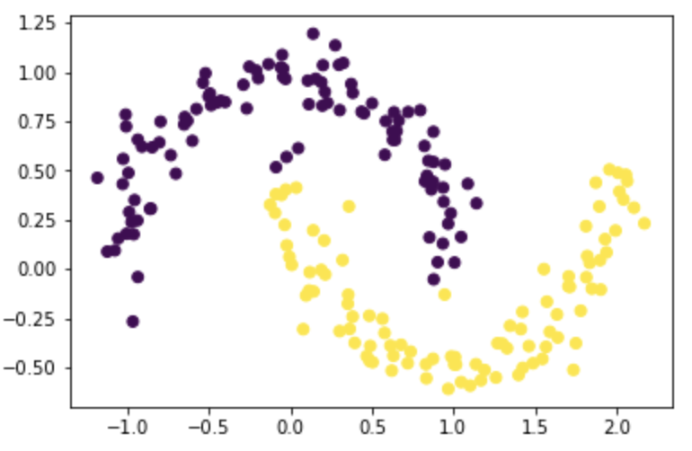
Test it on moons with noise=0.1:

X, y = datasets.make_moons(n_samples=n, shuffle=True, noise=0.1, random_state=None)
z_eig = spectral_clustering(X, epsilon)
plt.scatter(X[:,0], X[:,1], c=z_eig)

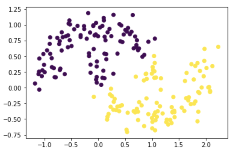
Test it on moons with noise=0.15:

X, y = datasets.make_moons(n_samples=n, shuffle=True, noise=0.15, random_state=None)
z_eig = spectral_clustering(X, epsilon)
plt.scatter(X[:,0], X[:,1], c=z_eig)

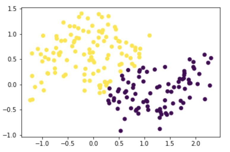
Test it on moons with noise=0.2:

X, y = datasets.make_moons(n_samples=n, shuffle=True, noise=0.2, random_state=None)
z_eig = spectral_clustering(X, epsilon)
plt.scatter(X[:,0], X[:,1], c=z_eig)

Test it on moons with noise=0.3 with n=1000:

n=1000
X, y = datasets.make_moons(n_samples=n, shuffle=True, noise=0.3, random_state=None)
z_eig = spectral_clustering(X, epsilon)
plt.scatter(X[:,0], X[:,1], c=z_eig)

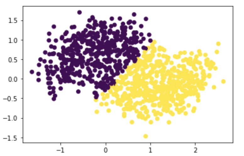
We can see that as noise increases, the moons created are gradually less similar to moon shapes, especially when noise is greater than 0.2. However, the algorithm still identifies two separated clusterings.

I. Challange!

Now let’s try our function on a more challenging dataset!

n, epsilon = 1000, 0.4
X, y = datasets.make_circles(n_samples=n, shuffle=True, noise=0.05, random_state=None, factor = 0.4)
z_eig = spectral_clustering(X, epsilon)
plt.scatter(X[:,0], X[:,1], c=z_eig)

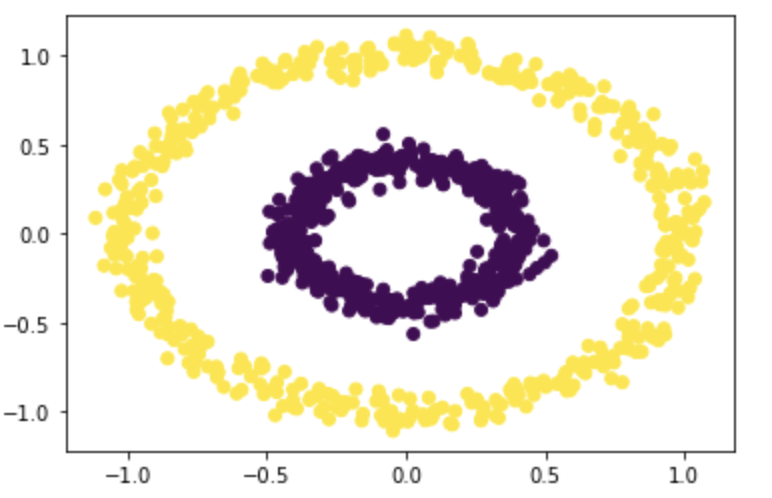
It works very well with epsilon=0.4! Let’s try it with some different epsilons:

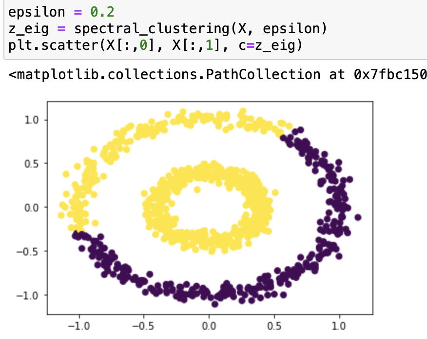
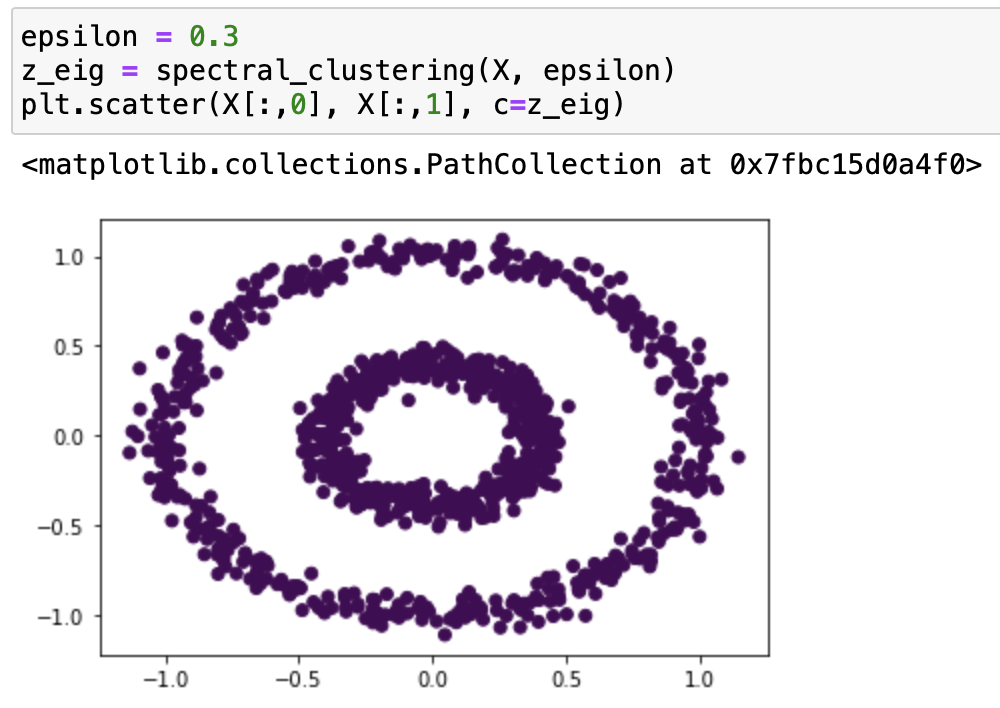
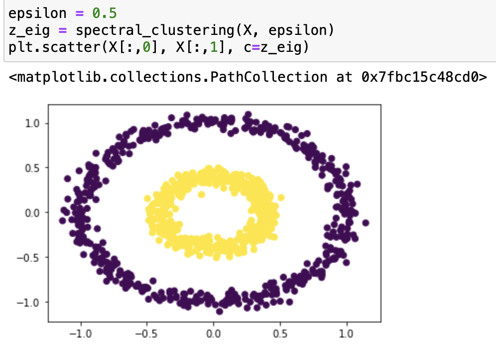
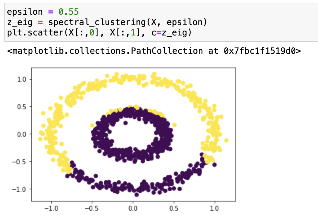
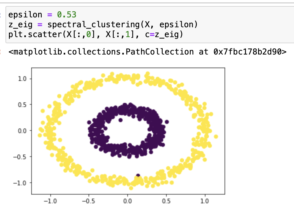
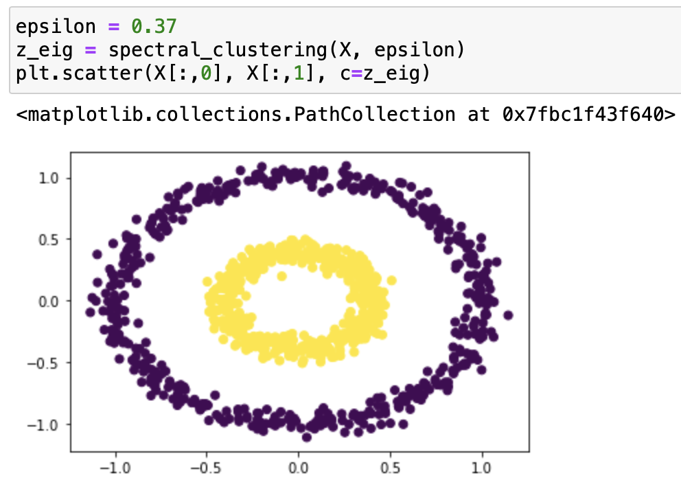
From our testing, we can see that it classifies epsilon=0.2, 0.3, 0.55 incorrectly, and 0.5, 0.37, 0.53 correctly. From the testing result we can say that this function works on bullseye with epsilons roughly from 0.37 to 0.53.